Spatial Statistics Toolbox 1.1
By
R. Kelley Pace
LREC Endowed Chair of Real Estate
E.J. Ourso College of Business Administration
Louisiana State University
Baton Rouge, LA 70803-6308
(225)-388-6256
FAX: (225)-334-1227
kelley@spatial-statistics.com
kelley@pace.am
www.spatial-statistics.com
and
Ronald Barry
Associate Professor of Statistics
Department of Mathematical Sciences
University of Alaska
Fairbanks, Alaska 99775-6660
(907)-474-7226
FAX: (907)-474-5394
FFRPB@uaf.edu
The authors gratefully acknowledge the research support they have received from the University of Alaska and Louisiana State University. We also wish to acknowledge support from the Center for Real Estate and Urban Studies at the University of Connecticut at Storrs. We would like to thank Jennifer Loftin for her editorial assistance as well as Rui Li, Sean McDonald, Robby Singh, and Dek Terrell for having made sure that the Toolbox could run on machines other than my own.
Spatial Statistics Toolbox
I. Why the Toolbox Exists
Many problems of practical importance generate large spatial data sets. Obvious examples include census data (over 200,000 block groups for the US) and housing sales (many millions sold per year). Almost any model fitted to these data will produce spatially correlated errors. Ignoring the spatial correlation among errors results in inefficient parameter estimation, biased inference, and ignores information which can greatly improve prediction accuracy.
Historically, spatial statistics software floundered with problems involving even thousands of observations. For example, Li (1995) required 8515 seconds to compute a 2,500 observation spatial autoregression using an IBM RS6000 Model 550 workstation. The culprit for the difficulty lies in the maximum likelihood estimator’s need for the determinant of the n by n matrix of the covariances among the spatially scattered observations.
The two most capable software packages which estimate these spatial autoregressions, SpaceStat and S+SpatialStats, improve upon the historical level of performance through the use of sparsity, simultaneously advocated by Barry and Pace (1997) and Pace and Barry (1997a,b, 1998). Dense matrices require O(n3) operations to compute determinants while sufficiently sparse matrices (large enough proportion of zeros) can require as few as O(n) operations to compute determinants. However, the commercial software packages do not fully exploit the advantages of sparsity (they ignore the reordering of the rows and columns which can greatly improve performance) and do not take advantage of some of the other techniques advocated in the Pace and Barry articles such as quick identification of neighboring observations, determinant reuse, the use of a grid of determinant values for direct computation of the full profile likelihood, and vectorizing the sum-of-squared error computations in the log-likelihood. Table 1, which compares the spatial statistics toolbox estimates and timings with those from S+SpatialStats provides a striking illustration of the potential gains of these techniques. For this data set of 3,107 observation with five variables and eight neighbors used in the computation of the inverse variance-covariance matrix, S+SpatialStats was slower than the Spatial Statistic Toolbox by a factor of 38.05. Specifically, it took 1304.83 seconds for S+SpatialStats to compute the estimates while it took only 34.29 seconds for the Spatial Statistics Toolbox (based on Matlab 5.2) to perform the same operation. The timings are on a dual Pentium Pro 200 Mhz computer with 256 megabytes of RAM. In passing, the Spatial Statistics Toolbox used much less memory (less than 64MB) than S-Plus (more than 128MB) in arriving at these results.
The Spatial Statistics Toolbox uses a grid of 100 values for the autoregressive parameter, a , for most of the maximum likelihood estimation and log-determinant functions. We restrict a to lie in [0,1) because almost all practical problems exhibit positive autocorrelation. The minor differences in the coefficient estimates arise due to the discrete approximation of the continuous a . Also, the spatial statistics toolbox, in line with its likelihood orientation, provides likelihood ratio (LR) as opposed to t statistics. This applies even to the OLS non-spatial routine.
Version 1.1 of the Spatial Statistics Toolbox adds two functions relating to the very nearest neighbor (or closest neighbor) spatial dependence. The log-determinant in this case has an amazingly simple form which permits development of a closed-form maximum likelihood spatial estimator. One function finds the closest neighbor and the other estimates a mixed regressive spatially autoregressive model using closest neighbor spatial dependence. It takes under 3.5 minutes to find the neighbors and estimate the model for a data set with 500,000 observations (Pentium III 500).
We have used these techniques to compute spatial autoregressions of over 500,000 observations and wish to provide others with the Spatial Statistics Toolbox to aid the widespread application of spatial statistics to large-scale projects. In addition, the toolbox can greatly help with simulations and other applications involving numerous estimations of spatial statistical data.
Table 1 — Splus and Spatial Toolbox Estimates and Timings for a SAR Estimate on a Problem with 3,107 Observations, 5 Variables, and 8 Neighbors (Splus reports asymptotic t tests, Spatial Toolbox reports Likelihood Ratio tests) |
||||
Bsplus |
tsplus |
Bspacetool |
-2LRspacetool |
|
| Intercept | 0.5178 | 9.1337 | 0.5164 | 77.84 |
| ln(Population > 18 years of Age) | -0.7710 | -35.1633 | -0.7707 | 1022.93 |
| ln(Population with Education > 12 years) | 0.2598 | 12.1428 | 0.2590 | 128.29 |
| ln(Owner Occupied Housing Units) | 0.4495 | 29.0240 | 0.4496 | 741.33 |
| ln(Aggregate Income) | 0.0129 | 0.5998 | 0.0132 | 0.38 |
| Optimal a | 0.7583 | not reported |
0.76 | 1321.23 |
| SSE | 34.4415 | 34.4212 | ||
| Median |e| | 0.0594 | 0.0594 | ||
| Log(Likelihood) | -5646 | -5646.46 | ||
| n | 3107 | 3107 | ||
| k | 5 | 5 | ||
| Number of Neighbors | 8 | 8 | ||
| Time to compute Nearest Neighbor Matrix | 27.83 | seconds |
2.47 | seconds |
| Time to compute Determinants | 29.84 | seconds | ||
| Time to compute SAR | 1.98 | seconds | ||
| Time to compute SAR and Determinants | 1277 | seconds |
||
| Total Time Needed | 1304.83 | seconds |
34.29 | seconds |
| Ratio of time S-Plus/Spatial Toolbox | 38.05 | times | ||
| Machine: Pentium Pro 200 dual | ||||
II. Using the Toolbox
A. Hardware and Software Requirements
The toolbox requires Matlab 5.0 or later. Unfortunately, previous editions of Matlab did not contain the Delaunay command and others needed for the toolbox. The total installation takes around 15 megabytes. The routines have been tested on PC compatibles — the routines should run on other platforms, but have not been tested on non-PC compatibles.
B. Installation
For users who can extract files from zip archives, follow the instructions for your product (e.g., Winzip) and extract the files into the directory in which you wish to install the toolbox. The installation program will create the following directory structure in whichever drive and directory you choose.
DRIVE:.
+---datasets
� +---geo_analysis
� +---harrison_rubinfeld
� +---statprob_letters
+---document
+---EXAMPLES
� +---XARY1
� +---XCAR1
� +---xclosestmix1
� +---XDELW1
� +---xh&r_data
� +---xlagx1
� +---xlagx2
� +---XMCCAR1
� +---XMCMIX1
� +---XMCPAR1
� +---XMCSAR1
� +---XMIX1
� +---XMIX2
� +---xnnasym1
� +---XNNDEL1
� +---xols1
� +---XPAR1
� +---xs&p_data
� +---XSAR1
+---FUNDIR
+---manuscripts
+---closest_neighbor
+---geo_analysis
+---JEEM
+---statistics_prob_lets
To see if the installation has succeeded, change the directory in Matlab to one of the supplied examples and type run "m-file name". For example, go to the ..\examples\xcar1 subdirectory and type run xcar1. This should cause the script xcar1.m containing the example to run. If it does not, check the file attributes as described below. All the example scripts should follow the form x*.m (e.g., xsar1.m, xols1.m). Functions follow the form f*.m (e.g., fsar1.m, fols1.m). Matlab matrix files (which may include multiple matrices) have the form *.mat. ASCII files have the form *.asc, text files have the form *.txt, postscript files have the form *.ps, Adobe Acrobat files have the form *.pdf, and html files naturally have the form *.html.
For non-PC platforms or if you have directly copied the files from the CD-ROM without using the installation program, it may still have the "read-only" file attribute. If so, change this manually. On the PC, for those who have not used the installation program, run Explorer, select the file menu, go to the Properties item, and you can change the file attributes this way. Again, this should not be a problem for those who used the installation program under Windows 95 or Windows NT. However, If the example fails, you should check to see if it has the "read-only" file attribute.
The examples that do not write to files can be run directly off the CD-ROM. For example, go to the stoolbox\examples\xcar1 subdirectory and type run xcar1. This should cause the script xcar1.m containing the CAR estimation example to run.
C. Using the Toolbox
Typical sessions with the toolbox proceed in four steps. First, import the data into Matlab, a fairly easy step. If the file is fixed-format or tab-delimited ASCII, load filename (whatever that filename may be) will load this into memory. Saving it will convert it into a matlab file (e.g., save a a will save variable a into matrix a — failure to specify both names will result in saving all defined variables into one file). The data would include the dependent variable, the independent variables, and the locational coordinates.
Second, create a spatial weight matrix. One can choose ones based upon nearest neighbors (symmetric or asymmetric) and Delaunay triangles (symmetric). In almost all cases, one must make sure each location is unique. One may need to add slight amounts of random noise to the locational coordinates to meet this restriction (some of the latest versions of Matlab do this automatically — do not dither the coordinates in this case). Note, some estimators only use symmetric matrices. You can specify the number of neighbors used and their relative weightings.
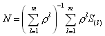
Note, the Delaunay spatial weight matrix leads to a concentration matrix or a variance-covariance matrix that depends upon only one-parameter (a , the autoregressive parameter). In contrast, the nearest neighbor concentration matrices or variance-covariance matrices depend upon three parameters (a , the autoregressive parameter; m, the number of neighbors; and r , which governs the rate weights decline with the order of the neighbors with the closest neighbor given the highest weighting, the second closest given a lower weighting, and so forth). Three parameters should make this specification sufficiently flexible for many purposes.
Third, one computes the log-determinants for a grid of autoregressive parameters (prespecified by the routine). We suggest the use of the determinant routines which interpolate to save time. The interpolation precision is very high relative to the statistical imprecision of the estimated SSE and should not affect the results. Determinant computations proceed faster for symmetric matrices. You must choose the appropriate log-determinant routines for the type of spatial weight matrix you have specified. Table 2 provides more detail on the relations among the routines. Computing the log-determinants is the slowest step but only needs to be done once for most problems (the same applies to creating the spatial weight matrix).
Table 2 — Relations Among Weight Matrix Routines, Log-Determinant Routines and Output |
|||
Weight Routines |
Log-Dets | Output | |
| Delaunay fdelw1 |
fdetfil1 or fdetinterp1 |
wswdel (symmetric Delaunay weight matrix) or wwsdel (similar row-stochastic weight matrix) and associated log-determinants detvalzdel | |
| Nearest
Neighbors Symmetric Weight Matrix fnndel1 (uses fdelw1) + fnnsym1 |
fdetfil1 or fdetinterp1 |
wswnn (symmetric NN weight matrix) or wwsnn (similar row-stochastic NN weight matrix) and associated log-determinants detvalznn | |
| Nearest
Neighbors Asymmetric Weight Matrix fnndel1 (uses fdelw1) + fnnasym1 |
fdetinterpasym1 | wwsnn (fundamentally asymmetric, row-stochastic NN weight matrix) and associated log-determinants detvalznn | |
Fourth, pick a statistical routine to run given the data matrices, the spatial weight matrix, and the log-determinant vector. One can choose among conditional autoregressions (CAR), simultaneous autoregressions (SAR), mixed regressive spatially autoregressive estimators, pure autoregressive estimators, spatially lagged independent variable models, and OLS. These routines require little time to run. One can change models, weightings, and transformations and reestimate in the vast majority of cases without rerunning the spatial weight matrix or log-determinant routines (you may need to add another simple Jacobian term when performing weighting or transformations). This aids interactive data exploration. The closest neighbor functions seem well-suited to exploratory work due to their speed. In addition, they provide an excellent naive model useful as a benchmark for more elaborate models.
Fifth, these procedures provide a wealth of information. Typically they yield the profile likelihood in the autoregressive parameter for each submodel (corresponding to the deletion of individual variables or pairs of a variable and its spatial lag). All of the inference, even for the OLS routine, uses likelihood ratio statistics. This facilitates comparisons among the different models. Note, the routines append the intercept as the last (as opposed to the usual first) variable.
D. Included Examples
The Spatial Statistics Toolbox comes with many examples. These are found in the subdirectories under ...\EXAMPLES. To run the examples, change the directory in Matlab into the many subdirectories that illustrate individual routines. Look at the documentation in each example directory for more detail. Almost all of the specific models have examples. In addition, the simulation routine examples serve as minor Monte Carlo studies which also help verify the functioning of the estimators. The examples use the 3,107 observation dataset from the Pace and Barry (1997) Geographical Analysis article.
E. Included Datasets
The ...\DATASETS subdirectory contains subdirectories with individual data sets in Matlab file formats as well as their documentation. One can obtain ascii versions of these data from the website www.spatial-statistics.com. The data sets include:
Table 3 — Included Data Sets and their Characteristics |
|||
n |
Dependent Variable |
Spatial Area |
Initial Appearances |
506 |
housing prices | Boston SMSA 1970 census tracts | Harrison and Rubinfeld
(1978), JEEM Gilley and Pace (1996), JEEM (added spatial coordinates to HR data) |
3,107 |
election turnout | US Counties | Pace and Barry (1997), Geographical Analysis |
20,640 |
housing prices | California Census Block Groups | Pace and Barry (1997), Statistics and Probability Letters |
The datasets also have example programs and output. Note, due to the many improvements incorporated into the Spatial Statistics Toolbox over time, the running times have greatly improved over those in the articles. For example, the California census block group data set with 20,640 observations now requires less than one minute to compute the spatial weight matrix, calculate the log-determinants, and to estimate the model. The original paper took around 19 minutes to perform just one estimate (given the weight matrix). Also, the original paper performed inference via t ratios conditional upon the autoregressive parameter while the new procedures yield likelihood ratio statistics for almost any hypothesis of interest. Table 4 shows typical time requirements for datasets of differing sizes.
Table 4 — Timings Across Datasets |
|||
| Time (in seconds) Needed to | Harrison and Rubinfeld Data (n=506) | Data used in Geographical Analysis Article (n=3,107) | Data used in Statistics and Probability Letters Article (n=20,640) |
| Create Delaunay weight matrix | 0.14 | 0.57 | 4.48 |
| Compute Interpolated Log-determinant | 3.41 | 6.36 | 44.86 |
| Estimate Mixed Regressive Spatially Autoregressive Model | 0.12 | 0.17 | 1.98 |
| Estimate SAR | 0.85 | 1.96 | 19.42 |
| Estimate CAR | 0.45 | 1.61 | 11.25 |
| Pentium 233Mhz machine | |||
Hopefully, these data sets should provide a good starting point for exploring applications of spatial statistics.
F. Included Manuscripts
In the manuscript subdirectory we provide html and postscript versions of the Geographical Analysis, Journal of Environmental and Economic Management (JEEM), and Statistics and Probability Letters articles. The copyrights for these articles are owned by the respective publishers. We thank the publishers for having given us copyright permission to distribute these works.
III. An Extremely Brief and Limited Introduction to Spatial Statistics
Much of the effort in spatial statistics has gone into modeling the dependence of
errors among different locations. The n by n variance-covariance matrix ![]() expresses such a dependence where
expresses such a dependence where ![]() represents the
covariance of the ith and jth errors. Ex-ante, the magnitude of the
covariance between any two errors
represents the
covariance of the ith and jth errors. Ex-ante, the magnitude of the
covariance between any two errors ![]() and
and ![]() declines as distance (given some metric) increases between location i
and location j. If the covariance depends strictly upon the distance between two
observations (relative position) and not upon their absolute position, the errors are isotropic.
Violation of this leads to anisotropy, a more difficult modeling problem. Just as
with time series, various forms of stationarity are important.
declines as distance (given some metric) increases between location i
and location j. If the covariance depends strictly upon the distance between two
observations (relative position) and not upon their absolute position, the errors are isotropic.
Violation of this leads to anisotropy, a more difficult modeling problem. Just as
with time series, various forms of stationarity are important.
The means of modeling the estimated variance-covariance matrix or functions of the estimated variance-covariance matrix and the method of prediction (BLUP or other method) distinguishes many of the strands of the spatial statistics literature.
Given an estimated variance-covariance matrix ![]() , one could compute
estimated generalized least squares (EGLS).
, one could compute
estimated generalized least squares (EGLS).
![]()
\* MERGEFORMAT ()1
The maximum likelihood estimate appears similar to EGLS but introduces a log-determinant term which penalizes the use of more singular estimated variance-covariance matrices (higher correlations among the observations cause the covariances (off-diagonal elements) to rise relative to the variances (diagonal elements) and this also makes the matrix more singular).
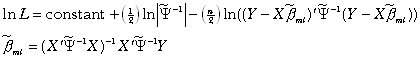
\* MERGEFORMAT ()2
If one uses a sum-of-squared error criteria alone in computing the estimates (e.g.,
use![]() ), this can lead to pathological results. Consider the extreme
but illustrative example of employing
), this can lead to pathological results. Consider the extreme
but illustrative example of employing ![]() comprised of all ones. Premultiplication of Y and X by this matrix would
result in a vector and a matrix of constants. The associated regression would display 0
error. Naturally,
comprised of all ones. Premultiplication of Y and X by this matrix would
result in a vector and a matrix of constants. The associated regression would display 0
error. Naturally, ![]() is singular in this case.
The log-determinant term correctly penalizes such singular transformations.
is singular in this case.
The log-determinant term correctly penalizes such singular transformations.
Misspecifying the variance-covariance matrix results in loss of efficiency, predictive accuracy, and biased inference. In the case of positive spatial autocorrelation, the OLS standard errors have a downward bias. Since the true information content in the spatially correlated observations is less than in the same number of independent observations, OLS overstates the precision of its estimates. Note, this statement may depend upon the mechanism which leads to spatial autocorrelation. If the observed autocorrelation arises due to omitted variables or misspecification, the parameter estimates may be inconsistent relative to the perfectly specified model. Note, the maximum likelihood spatial model has an instrumental variable interpretation. To see this write the maximum likelihood estimator in as,
![]()
\* MERGEFORMAT ()3
where Z represents the instrumental variables (Pace and Gilley (1998)). To the degree the spatial transformations construct good instruments, one suspects some of the favorable bias properties of instrumental variable estimators may carry through. Finally, for individual estimates for a given dataset, inefficiency can be just as fatal as bias.
Prediction with correlated data becomes somewhat more complex than for the independent observation case. The best linear unbiased predictor (BLUP) for the case of spatial correlation and no measurement error equals,
![]()
\* MERGEFORMAT ()4
where ![]() represents an n by 1 vector
of covariances between the error for observation o and the errors on the sample
observations. If no measurement error exists and
represents an n by 1 vector
of covariances between the error for observation o and the errors on the sample
observations. If no measurement error exists and ![]() is ith
sample observation, the prediction will be exactly equal to the sample value
is ith
sample observation, the prediction will be exactly equal to the sample value![]() and hence the method produces identically 0 errors for sample
observations. This occurs because the covariance vector multiplied by the inverse
covariance matrix will result in a vector of all zeros except for a 1 in the ith
position and hence
and hence the method produces identically 0 errors for sample
observations. This occurs because the covariance vector multiplied by the inverse
covariance matrix will result in a vector of all zeros except for a 1 in the ith
position and hence ![]() . Thus, BLUP for the case of spatial correlation
with no measurement error produces an exact interpolator — 0 error at each sample
observation.
. Thus, BLUP for the case of spatial correlation
with no measurement error produces an exact interpolator — 0 error at each sample
observation.
In the case of pure measurement error with no spatial autocorrelation, the BLUP becomes
the familiar ![]() . In the case of measurement error and spatial
autocorrelation, the BLUP becomes a smoothing and not an exact interpolation procedure at
the sample points. Conditional autoregression (CAR) predictions can be BLUP under this
these conditions. Simultaneous autoregressions (SAR) predictions are not BLUP, but do use
the correlation structure to improve prediction. The SAR predictions resemble those used
from semiparametric (with space as the nonparametric component) estimators. Mixed
regressive spatially autoregressive models also fall into this category. Table 5 provides
a brief annotated bibliography of some easy-to-read materials as well as reference
resources. The bibliography provides additional references.
. In the case of measurement error and spatial
autocorrelation, the BLUP becomes a smoothing and not an exact interpolation procedure at
the sample points. Conditional autoregression (CAR) predictions can be BLUP under this
these conditions. Simultaneous autoregressions (SAR) predictions are not BLUP, but do use
the correlation structure to improve prediction. The SAR predictions resemble those used
from semiparametric (with space as the nonparametric component) estimators. Mixed
regressive spatially autoregressive models also fall into this category. Table 5 provides
a brief annotated bibliography of some easy-to-read materials as well as reference
resources. The bibliography provides additional references.
A. Lattice Models
A set of observations located on a plane forms a lattice. Lattice models directly
approximate ![]() in the case of conditional
autoregressions or
in the case of conditional
autoregressions or ![]() in the case of
simultaneous autoregressions or models with lagged spatial dependent variables. The CAR
model usually specifies
in the case of
simultaneous autoregressions or models with lagged spatial dependent variables. The CAR
model usually specifies ![]() and SAR specifies
and SAR specifies ![]() ,
where C, D represent spatial weight matrices and
,
where C, D represent spatial weight matrices and ![]() represent the relevant autoregressive parameters. Positive
represent the relevant autoregressive parameters. Positive ![]() correspond to asserting that some form of direct dependency exists
between observation i and j. One can determine which
correspond to asserting that some form of direct dependency exists
between observation i and j. One can determine which ![]() >0 through cardinal distance or through ordinal distance (e.g.,
the eight closest neighbors). Typically, C and D have zeros on the diagonal
and are non-negative matrices. In addition, C must possess symmetry. The zeros on
the diagonal means that observations are not used to predict themselves. Hence, lattice
models do not attempt to exactly interpolate (exhibit zero error at all the sample
points).
>0 through cardinal distance or through ordinal distance (e.g.,
the eight closest neighbors). Typically, C and D have zeros on the diagonal
and are non-negative matrices. In addition, C must possess symmetry. The zeros on
the diagonal means that observations are not used to predict themselves. Hence, lattice
models do not attempt to exactly interpolate (exhibit zero error at all the sample
points).
Often the rows of D sum to 1 (row-stochastic) which gives them a filtering
interpretation. Hence, DY would contain the average value of the neighboring Y
for each observation. For row-stochastic matrices, the log-determinants ![]() will be defined for autoregressive parameters
less than 1. Also, matrices similar (in the linear algebra sense) to these will have the
same eigenvalues and hence log-determinants. If one begins from a symmetric matrix, one
can reweight this to form either a symmetric matrix with a maximum eigenvalue of 1 or a
similar row-stochastic matrix with a maximum eigenvalue of 1. Ord (1975) discussed the
similarity between the row-stochastic weighting of a symmetric matrix and a symmetric
weighting of the same matrix. Pace and Barry (1998) discuss this in more detail. As
log-determinants are easier to compute for symmetric matrices, the toolbox may use
symmetric matrices to compute the log-determinants and use the similar row-stochastic
matrix for estimation.
will be defined for autoregressive parameters
less than 1. Also, matrices similar (in the linear algebra sense) to these will have the
same eigenvalues and hence log-determinants. If one begins from a symmetric matrix, one
can reweight this to form either a symmetric matrix with a maximum eigenvalue of 1 or a
similar row-stochastic matrix with a maximum eigenvalue of 1. Ord (1975) discussed the
similarity between the row-stochastic weighting of a symmetric matrix and a symmetric
weighting of the same matrix. Pace and Barry (1998) discuss this in more detail. As
log-determinants are easier to compute for symmetric matrices, the toolbox may use
symmetric matrices to compute the log-determinants and use the similar row-stochastic
matrix for estimation.
Lattice models have close analogs in time series. For example, SAR models subtract the
average of the surrounding observations (scaled by the autoregressive parameter ![]() ) from each observation. This resembles the
operation in time series for an AR(1) process of subtracting from an observation the
previous observation scaled by an autoregressive constant (e.g.,
) from each observation. This resembles the
operation in time series for an AR(1) process of subtracting from an observation the
previous observation scaled by an autoregressive constant (e.g., ![]() ,
, ![]() ). As the log-determinant is equal to 0 when
dealing strictly with past data, this term does not present the same challenge for time
series analysis as it does for spatial statistics. However, spatial statistics has the
advantage of having observations in different directions near each observation while time
series always deals with purely past data. Hence, the greater symmetry and additional
observations around each observation aids spatial statistics in prediction relative to the
fundamental asymmetry of time series analysis.
). As the log-determinant is equal to 0 when
dealing strictly with past data, this term does not present the same challenge for time
series analysis as it does for spatial statistics. However, spatial statistics has the
advantage of having observations in different directions near each observation while time
series always deals with purely past data. Hence, the greater symmetry and additional
observations around each observation aids spatial statistics in prediction relative to the
fundamental asymmetry of time series analysis.
B. Geostatistical Models
Effectively, geostatistical models directly estimate the variance-covariance matrix.
Geostatistical techniques, such as kriging (named after Krige, a South African mining
engineer) rely upon an estimated variance-covariance matrix, ![]() ,
followed by EGLS (estimated generalized least squares), and BLUP (best linear unbiased
prediction). The simplest case assumes one can specify correctly the variance-covariance
matrix as a function of distance only (isotropy). The most typical application involves
the smooth interpolation of a surface at points other than those measured. Usually, the
method assumes errors are 0 at the measured points but modifications allow for measurement
errors at the sample points (nugget effect).
,
followed by EGLS (estimated generalized least squares), and BLUP (best linear unbiased
prediction). The simplest case assumes one can specify correctly the variance-covariance
matrix as a function of distance only (isotropy). The most typical application involves
the smooth interpolation of a surface at points other than those measured. Usually, the
method assumes errors are 0 at the measured points but modifications allow for measurement
errors at the sample points (nugget effect).
IV. Conclusion and Future Plans
The spatial statistics toolbox provides very rapid maximum likelihood estimation and likelihood-based inference for a variety of models (with a heavy emphasis upon lattice models). The toolbox particularly excels at spatial estimation with large data sets. The slow parts of the estimation (log-determinants) are usually run only once and subsequent interactions with the data and models require little time. This aids experimentation with spatial estimation, a goal of the Toolbox. Use of the closest neighbor functions (which uses a closed-form log-determinant formula) can provide benchmarks useful in assessing the contribution of more elaborate models.
At the moment the toolbox does not include any geostatistical routines. We have some of these, but we wish to refine these to increase the level of performance before adding them to the toolbox.
We also have routines to estimate the log-determinant, a procedure which can save great amounts of time for large matrices. We described the algorithm in Barry, Ronald, and R. Kelley Pace, "A Monte Carlo Estimator of the Log Determinant of Large Sparse Matrices," Linear Algebra and its Applications, Volume 289, Number 1-3, 1999, p. 41-54. We may wish to later add some spatio-temporal estimation routines which we presented in Pace, R. Kelley, Ronald Barry, John Clapp, and M. Rodriguez, (1998), "Spatio-Temporal Estimation of Neighborhood Effects," Journal of Real Estate Finance and Economics. Naturally, we have current research projects which will augment the present set of routines. We plan to provide additional datasets as well.
We welcome any comments you might have. We hope you will find these routines useful and encourage others to use these. If you would like to keep current on this product or any other spatial statistics software product we provide (e.g., we have a some of these routines available in Fortran 90 source code with PC executable files, a product we call SpaceStatPack), you might examine our web site at www.spatial-statistics.com from time to time. We have the latest version of this product there available for downloading. If you use the product, please send an email message to either kelley@spatial-statistics.com with the first word in the subject field as "spacetoolbox" which will allow us to do a quick search to form a mailing list when we wish to communicate with interested individuals. We will try to assist individuals interested in using the toolbox. However, we request you read the documentation and experiment with the product before requesting help. We do not charge for the product and so cannot afford to provide extensive support. If you need extensive support, you probably should pay for one of the commercial products. These have more extensive documentation, have undergone more testing, and provide on-going technical support.
Table 5 — Some Spatial Statistics Selections |
|
| Anselin (1988) | This provides the most detailed exposition of simultaneously specified lattice models from a geographic and econometric perspective. |
| Anselin and Hudak (1992) | Good description of the basic estimation problem. This appears in a special issue containing a number of interesting articles. |
| Bailey and Gatrell (1995) | Albeit limited, this is the easiest introduction to the various spatial statistical methods. As a bonus, the text comes with DOS software for estimating some of the models. |
| Besag (1975) | A clear exposition of the conditional approach. |
| Christensen (1991) | Provides an easy-to-read discussion of kriging with measurement error. |
| Cressie (1993) | This voluminous text treats both lattice and geostatistical models and serves as a standard reference for the field. |
| Dubin (1988) | This provides one of the clearest expositions of spatial statistical estimation. |
| Goldberger (1962) | The easiest-to-read derivation of best linear unbiased prediction (BLUP) from an econometric perspective and notation. |
| Griffith (1992) | An interesting, non-technical discussion of the various causes and implications of spatial autocorrelated data. |
| Haining (1990) | A well-written, comprehensive survey of the field. Inexpensive. |
| Ord (1975) | A starting point for simultaneous geographical lattice modeling. |
| Ripley (1981) | This develops SAR and CAR lattice models as well as geostatistical ones. A standard reference in the field. |
References
Anselin, Luc. (1988) Spatial Econometrics: Methods and Models. Dordrecht: Kluwer Academic Publishers.
Anselin, Luc, and S. Hudak. (1992) "Spatial Econometrics in Practice: A Review of Software Options," Journal of Regional Science and Urban Economics 22, 509-536.
Anselin, Luc. (1995) SpaceStat Version 1.80 User’s Guide, Morgantown WV: Regional Research Institute at West Virginia University.
Bailey, T., and A. Gatrell. (1995) Interactive Spatial Data Analysis. Harlow. Longman.
Barry, Ronald, and R. Kelley Pace. (1997) "Kriging with Large Data Sets Using Sparse Matrix Techniques," Communications in Statistics: Computation and Simulation 26, 619-629.
Barry, Ronald, and R. Kelley Pace, "A Monte Carlo Estimator of the Log Determinant of Large Sparse Matrices," Linear Algebra and its Applications, Volume 289, Number 1-3, 1999, p. 41-54.
Belsley, David, Edwin Kuh, and Roy Welsch. (1980) Regression Diagnostics. New York. Wiley.
Besag, J. E. (1974) "Spatial Interaction and the Statistical Analysis of Lattice Systems," Journal of the Royal Statistical Society, B, 36, p. 192-225.
Besag, J. E. (1975) "Statistical Analysis of Non-lattice Data," The Statistician, 24, p. 179-195.
Christensen, Ronald. (1991) Linear Models for Multivariate, Time Series, and Spatial Data. New York: Springer-Verlag.
Cressie, Noel A.C. (1993) Statistics for Spatial Data, Revised ed. New York. John Wiley.
Dubin, Robin A. (1988) "Estimation of Regression Coefficients in the Presence of Spatially Autocorrelated Error Terms," Review of Economics and Statistics 70, 466-474.
Dubin, Robin A., R. Kelley Pace, and Thomas Thibodeau. (forthcoming) "Spatial Autoregression Techniques for Real Estate Data," Journal of Real Estate Literature.
Gilley, O.W., and R. Kelley Pace. (1996) "On the Harrison and Rubinfeld Data," Journal of Environmental Economics and Management, 31, 403-405.
Goldberger, Arthur. (1962) "Best Linear Unbiased Prediction in the Generalized Linear Regression Model," Journal of the American Statistical Association, 57, 369-375.
Griffith, Daniel A. (1992) "What is Spatial Autocorrelation?," L’Espace G�ographique 3, 265-280.
Haining, Robert. (1990) Spatial Data Analysis in the Social and Environmental Sciences. Cambridge.
Harrison, David, and Daniel L. Rubinfeld. (1978) "Hedonic Housing Prices and the Demand for Clean Air," Journal of Environmental Economics and Management, Volume 5, 81-102.
Kaluzny, Stephen, Silvia Vega, Tamre Cardoso, and Alice Shelly. (1996) S+SPATIALSTATS User’s Manual Version 1.0, Seattle: Mathsoft.
Kelejian, Harry and Igmar Prucha. (1998) "A Generalized Spatial Two Stage Least Squares Procedure for Estimating a Spatial Autoregressive Model with Autoregressive Disturbances,"17, Journal of Real Estate Finance and Economics.
Li, Bin. (1995) "Implementing Spatial Statistics on Parallel Computers," in: Arlinghaus, S., ed. Practical Handbook of Spatial Statistics (CRC Press, Boca Raton), pp. 107-148.
Ord, J.K. (1975). "Estimation Methods for Models of Spatial Interaction," Journal of the American Statistical Association 70, 120-126.
Pace, R. Kelley, and Ronald Barry. (1998) "Simulating Mixed Regressive Spatially Autoregressive Estimators," Computational Statistics 13, 397-418.
Pace, R. Kelley, and Ronald Barry. (1997) "Fast CARs," Journal of Statistical Computation and Simulation 59, p. 123-147.
Pace, R. Kelley, Ronald Barry, and C.F. Sirmans. (1998) "Spatial Statistics and Real Estate," 17, Journal of Real Estate Finance and Economics.
Pace, R. Kelley, and Ronald Barry. (1997) "Quick Computation of Regressions with a Spatially Autoregressive Dependent Variable," Geographical Analysis 29, 232-247.
Pace, R. Kelley, and O.W. Gilley. (1997) "Using the Spatial Configuration of the Data to Improve Estimation," Journal of the Real Estate Finance and Economics 14, 333-340.
Pace, R. Kelley, and O.W. Gilley. (1998) "Optimally Combining OLS and the Grid Estimator," Real Estate Economics, 26, p. 331-347.
Pace, R. Kelley, and Ronald Barry. (1997) "Sparse Spatial Autoregressions," Statistics and Probability Letters, 33, 291-297.
Pace, R. Kelley, Ronald Barry, John Clapp, and M. Rodriguez. (1998) "Spatio-Temporal Estimation of Neighborhood Effects," 17, Journal of Real Estate Finance and Economics.
Pace, R. Kelley, and Dongya Zou. (forthcoming), "Closed-Form Maximum Likelihood Estimates of Nearest Neighbor Spatial Dependence," Geographical Analysis.
Ripley, Brian D. (1981) Spatial Statistics. New York. John Wiley.
Spatial Statistics Toolbox Reference
Spatial Weight Matrix Functions
fclosestnn1.m – Finds closest neighbor to each observation.
fdelw1.m – Creates spatial weight matrix using Delaunay triangles.
fnndel1.m – Creates individual neighbor weight matrices from first and second order Delaunay neighbors.
fnnsym1.m – Takes individual neighbor weight matrices, smats, and forms overall symmetric weight matrices.
fnnasym1.m – Takes individual neighbor weight matrices, smats, and forms overall asymmetric weight matrices.
Spatial Jacobian Computations
fdetfil1.m – Computes ln|I-aD| where D is a symmetric spatial weight matrix.
fdetinterp1.m – like fdetfil1.m, but uses spline interpolation to reduce determinant computations.
fdetinterpasym1.m – like fdetinterp1 but handles asymmetric weight matrices.
Spatial Autocorrelation Testing
fary1.m – Rapidly computes ML for Y=intercept+alpha*Y+e. This can work with a single vector or collection of vectors.
Lattice Model Estimation Functions
fcar1.m – Computes Maximum Likelihood Estimates for CAR errors.
fclosestmix1.m – Computes Closed-Form Maximum Likelihood Estimates when using only the nearest neighbor.
fsar1.m – Computes Maximum Likelihood Estimates for SAR errors.
fmix1.m – Computes Maximum Likelihood SAR estimates with spatially lagged X and Y.
fpar1.m – Computes Maximum Likelihood SAR estimates with spatially lagged Y but not spatially lagged X.
flagx1.m – Computes Maximum Likelihood SAR estimates with spatially lagged X, likelihood ratios for hypothesis that a variable and its spatial lag have no effect.
flagx2.m – Computes Maximum Likelihood SAR estimates with spatially lagged X, likelihood ratios for hypothesis that each individual variable (lagged or not lagged) has no effect.
Lattice Model Simulation Functions
fsimcar1.m – Simulates CAR random variables.
fsimsar1.m – Simulates SAR random variables.
fsimmix1.m – Simulates Mixed and Pure SAR random variables.
Non-spatial Estimation Functions
fols1.m – Computes OLS with likelihood ratios in the same form as fcar1, fsar1, etc.
FARY1
Syntax
[alphamax,loglik,emax,bmax,likratios,prhigher]=fary1(y,detvalz,wws)
Input Arguments
| y | n by q matrix containing observations on the q dependent variable series |
| detvalz | iter by 2 matrix
containing the grid of values for the autoregressive parameter a
in column 1 and the associated values of |
| wws | row-stochastic n by n spatial weighting matrix |
Output Arguments
| alphamax | |
| loglik | iter by q matrix of profile likelihoods over the iter grid of values for a . Each column is the unrestricted model profile log-likelihood for that series |
| emax | n by q matrix of AR errors with each column corresponding to one of the q series |
| bmax | q element vector
with each element representing the average of |
| likratios | q element vector of twice difference between the unrestricted log-likelihood from the overall model and the log-likelihood for a =0 (e.g., the restricted model is OLS or the sample average for each series). Hence, this is really the deviance (-2log(LR)). Individually these have a chi-squared distribution with 1 degree-of-freedom under the null hypothesis of no effect. |
| prhigher | q element vector of the probability of obtaining a higher chi-squared test statistic under the null hypothesis of no effect. |
Description
For a n element vector of observations on the dependent variable, ![]() (for j=1...q), this function fits the simple
autoregressive model
(for j=1...q), this function fits the simple
autoregressive model ![]() via maximum likelihood. This function can
handle q vectors at the same time by supplying a matrix of observations on the q
dependent variables. One could use this as a way of testing for autocorrelation for any
given variable or set of variables. In other words, this provides a maximum likelihood
alternative to estimators like the Moran’s I.
via maximum likelihood. This function can
handle q vectors at the same time by supplying a matrix of observations on the q
dependent variables. One could use this as a way of testing for autocorrelation for any
given variable or set of variables. In other words, this provides a maximum likelihood
alternative to estimators like the Moran’s I.
FCAR1
Syntax
[alphamax,loglik,emax,bmax,likratios,prhigher]=fcar1(xsub,y,detvalz,wsw)
Input Arguments
| xsub | n by p matrix where n represents the number of observations and p represents the number of non-constant independent variables |
| y | n element vector containing observations on the dependent variable |
| detvalz | iter by 2 matrix
containing the grid of values for the autoregressive parameter a
in column 1 and the associated values of |
| wsw | Symmetric n by n spatial weighting matrix |
Output Arguments
| alphamax | |
| loglik | iter by (k+1) matrix of profile likelihoods over the iter grid of values for a . The first column is the unrestricted model profile log-likelihood followed by the respective delete-1 variable subset restricted profile log-likelihoods |
| emax | n element vector of the errors from CAR prediction |
| bmax | k element vector of CAR parameter estimates |
| likratios | k element vector of twice difference between the unrestricted log-likelihood from the overall model and the k delete-1 variable subset restricted log-likelihoods. Hence, this is really the deviance (-2log(LR)). Individually these have a chi-squared distribution with 1 degree-of-freedom under the null hypothesis of no effect. |
| prhigher | k element vector of the estimated probability of obtaining a higher chi-squared test statistic under the null hypothesis of no effect. |
Description
For the conditional autoregression model (CAR), ![]() where D
represents an n by n symmetric matrix with zeros on the diagonal and
non-negative elements elsewhere. The CAR prediction is
where D
represents an n by n symmetric matrix with zeros on the diagonal and
non-negative elements elsewhere. The CAR prediction is ![]() and hence
and hence ![]() .
.
FCLOSESTMIX1
Syntax
[alphamax,loglik,emax,bmax,likratios,prhigher]=fclosestmix1(xsub,y,nnlist)
Input Arguments
| xsub | n by p matrix where n represents the number of observations and p represents the number of non-constant independent variables |
| y | n element vector containing observations on the dependent variable |
| nnlist | n element permutation vector which gives row number of the closest neighbor |
Output Arguments
| alphamax | |
| loglik | iter by (k+1) matrix of profile likelihoods over the iter grid of values for a . The first column is the unrestricted model profile log-likelihood, followed by p respective delete-2 variable subset restricted profile log-likelihoods (variable and its spatial lag), and ending with the no intercept restricted profile log-likelihood |
| emax | n element vector of the errors from mixed model prediction |
| bmax | 2p+1 element vector of mixed regressive spatially autoregressive model parameter estimates |
| likratios | k element vector of twice difference between the unrestricted log-likelihood from the overall model and the subset restricted log-likelihoods. For the non-constant variables the relevant restricted model corresponds to deleting a variable and its spatial lag. Therefore, this is really the deviance (-2log(LR)). Hence, these have a chi-squared distribution with 2 degree-of-freedom under the null hypothesis of no effect. The no intercept hypothesis has 1 degree-of-freedom. |
| prhigher | k element vector of the estimated probability of obtaining a higher chi-squared test statistic under the null hypothesis of no effect. |
Description
This function fits the model ![]() where D a spatial weight
matrix using only the closest neighbor. The mixed model prediction is
where D a spatial weight
matrix using only the closest neighbor. The mixed model prediction is ![]() . This uses the closed-form maximum likelihood method proposed by Pace
and Zou (forthcoming).
. This uses the closed-form maximum likelihood method proposed by Pace
and Zou (forthcoming).
FCLOSESTNN1PC
Syntax
[nnlist]=fclosestnn1pc(xcoord,ycoord)
Input Arguments
| xcoord | n by 1 vector of x coordinates such as longitude or from some projection |
| ycoord | n by 1 vector of y coordinates such as latitude or from some projection |
Output Arguments
| nnlist | n element permutation vector which gives row number of the closest neighbor |
Description
This routine finds the very nearest or closest neighbor using a Delaunay based method. It requires somewhat less memory and time than finding the nearest neighbors and extracting the closest one.
FDELW1
Syntax
[wswdel,wwsdel,wmatdel]=fdelw1(xcoord,ycoord)
Input Arguments
| xcoord | n by 1 vector of x coordinates such as longitude or from some projection |
| ycoord | n by 1 vector of y coordinates such as latitude or from some projection |
Output Arguments
| wswdel | Symmetric n by n sparse spatial weighting matrix |
| wwsdel | Row-stochastic n by n sparse spatial weighting matrix similar to wswdel |
| wmatdel | Diagonal n by n sparse matrix used to normalize a binary weighting matrix so the maximum eigenvalue equals one |
Description
This function computes Delaunay triangles and from these creates a binary sparse spatial weighting matrix with ones for observations connected by a side of one of the triangles. It subsequently takes the binary weighting matrix and computes two other weighting matrices. The first, wswdel, is symmetric with a maximum eigenvalue of 1. The second, wwsdel, is row-stochastic (rows sum to 1) and has a maximum eigenvalue of 1. The routine uses wmatdel to reweight these alternative forms. Specifically,
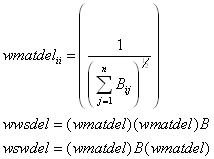
where B represents the binary spatial weighting matrix. As both wwsdel and wswdel have the same eigenvalues (see Ord (JASA, 1975)), using one form or another in a particular circumstance may have advantages. For example, using the symmetric form wswdel saves time in computing the log-determinants while using the row-stochastic form wwsdel has some nice smoothing interpretations (the row-stochastic form constitutes a two-dimensional linear filter). Both wwsdel and wswdel are quite sparse — there should be no more than 6 non-zero entries on average in each row. However, the maximum number of entries in a particular row could be fairly large.
FDETFIL1
Syntax
[detvalz]=fdetfil1(wsw)
Input Arguments
| wsw | Symmetric n by n spatial weighting matrix |
Output Arguments
| detvalz | iter by 2 matrix
containing the grid of values for the autoregressive parameter a
in column 1 and the associated values of |
Description
Computes ![]() over a grid for
over a grid for ![]() (which has iter elements). The routine uses the symmetric weighting
matrix, wsw, in the computations. However, this has the same log-determinants as the similar
row-stochastic wws.
(which has iter elements). The routine uses the symmetric weighting
matrix, wsw, in the computations. However, this has the same log-determinants as the similar
row-stochastic wws.
FDETINTERP1
Syntax
[detvalz]=fdetinterp1(wsw)
Input Arguments
| wsw | Symmetric n by n spatial weighting matrix |
Output Arguments
| detvalz | iter by 2 matrix
containing the grid of values for the autoregressive parameter a
in column 1 and the associated values of |
Description
Computes ![]() over a grid for
over a grid for ![]() (which has iter elements). Uses the symmetric weighting matrix, wsw, in the
computations. However, this has the same log-determinants as the similar row-stochastic wws. Uses spline
interpolation to reduce the number of determinant computations with very little loss in
accuracy.
(which has iter elements). Uses the symmetric weighting matrix, wsw, in the
computations. However, this has the same log-determinants as the similar row-stochastic wws. Uses spline
interpolation to reduce the number of determinant computations with very little loss in
accuracy.
FDETINTERPASYM1
Syntax
[detvalz]=fdetinterpasym1(wws)
Input Arguments
| wws | Asymmetric n by n spatial weighting matrix (not similar to a symmetric matrix) |
Output Arguments
| detvalz | iter by 2 matrix
containing the grid of values for the autoregressive parameter a
in column 1 and the associated values of |
Description
Computes ![]() over a grid for
over a grid for ![]() (which has iter elements). Uses the asymmetric weighting matrix, wws, in the
computations.
(which has iter elements). Uses the asymmetric weighting matrix, wws, in the
computations.
FLAGX1
Syntax
[alphamax,loglik,emax,bmax,likratios,prhigher]=flagx1(xsub,y,wws)
Input Arguments
| xsub | n by p matrix where n represents the number of observations and p represents the number of non-constant independent variables |
| y | n element vector containing observations on the dependent variable |
| wws | n by n spatial weighting matrix |
Output Arguments
| alphamax | 0 by definition |
| loglik | (k+1) vector of log-likelihoods. The first column is the unrestricted model log-likelihood, followed by p respective delete-2 variable subset restricted log-likelihoods (variable and its spatial lag), and ending with the no intercept restricted log-likelihood |
| emax | n element vector of the errors from OLS prediction with spatially lagged independent variables in the model |
| bmax | 2p+1 element vector of model parameter estimates |
| likratios | k element vector of twice difference between the unrestricted log-likelihood from the overall model and the subset restricted log-likelihoods. Hence, this is really the deviance (-2log(LR)). For the non-constant variables the relevant restricted model corresponds to deleting a variable and its spatial lag. Therefore, these have a chi-squared distribution with 2 degree-of-freedom under the null hypothesis of no effect. The no intercept hypothesis has 1 degree-of-freedom. |
| prhigher | k element vector of the estimated probability of obtaining a higher chi-squared test statistic under the null hypothesis of no effect. |
Description
This function fits the model ![]() where D represents an n
by n spatial weight matrix. Usually, one would employ a row-stochastic spatial
weight matrix which gives this the interpretation of regressing the dependent variable on
the independent variables and their local, spatial averages. The prediction is
where D represents an n
by n spatial weight matrix. Usually, one would employ a row-stochastic spatial
weight matrix which gives this the interpretation of regressing the dependent variable on
the independent variables and their local, spatial averages. The prediction is ![]() . This function provides for likelihood ratio tests for the sub-models
associated with the deletion of a variable and its associated spatial lag (with the
exception of the intercept variable). It differs in this respect from flagx2.
. This function provides for likelihood ratio tests for the sub-models
associated with the deletion of a variable and its associated spatial lag (with the
exception of the intercept variable). It differs in this respect from flagx2.
FLAGX2
Syntax
[alphamax,loglik,emax,bmax,likratios,prhigher]=flagx2(xsub,y,wws)
Input Arguments
| xsuby | n element vector containing observations on the dependent variable | |
| wws | n by n spatial weighting matrix | |
Output Arguments
| alphamax | 0 by definition |
| loglik | 2(p+1) vector of log-likelihoods. The first column is the unrestricted model log-likelihood, followed by p respective delete-1 variable subset restricted log-likelihoods (variable and its spatial lag), and ending with the no intercept restricted log-likelihood |
| emax | n element vector of the errors from OLS prediction with spatially lagged independent variables in the model |
| bmax | 2p+1 element vector of mixed model parameter estimates |
| likratios | 2p+1 element vector of twice difference between the unrestricted log-likelihood from the overall model and the delete-1 subset restricted log-likelihoods. Hence, this is really the deviance (-2log(LR)). Therefore, these have a chi-squared distribution with 1 degree-of-freedom under the null hypothesis of no effect. |
| prhigher | 2p+1 element vector of the estimated probability of obtaining a higher chi-squared test statistic under the null hypothesis of no effect. |
Description
This function fits the model ![]() where D represents an n
by n spatial weight matrix. Usually, one would employ a row-stochastic spatial
weight matrix which gives this the interpretation of regressing the dependent variable on
the independent variables and their local, spatial averages. The prediction is
where D represents an n
by n spatial weight matrix. Usually, one would employ a row-stochastic spatial
weight matrix which gives this the interpretation of regressing the dependent variable on
the independent variables and their local, spatial averages. The prediction is ![]() . This function provides likelihood ratio test statistics for all
delete-1 sub-models. It differs in this respect from flagx1.
. This function provides likelihood ratio test statistics for all
delete-1 sub-models. It differs in this respect from flagx1.
FMIX1
Syntax
[alphamax,loglik,emax,bmax,likratios,prhigher]=fmix1(xsub,y,detvalz,wws)
Input Arguments
| xsub | n by p matrix where n represents the number of observations and p represents the number of non-constant independent variables |
| y | n element vector containing observations on the dependent variable |
| detvalz | iter by 2 matrix
containing the grid of values for the autoregressive parameter a
in column 1 and the associated values of |
| wws | n by n spatial weighting matrix (usually row-stochastic) |
Output Arguments
| alphamax | |
| loglik | iter by (k+1) matrix of profile likelihoods over the iter grid of values for a . The first column is the unrestricted model profile log-likelihood, followed by p respective delete-2 variable subset restricted profile log-likelihoods (variable and its spatial lag), and ending with the no intercept restricted profile log-likelihood |
| emax | n element vector of the errors from mixed model prediction |
| bmax | 2p+1 element vector of mixed model parameter estimates |
| likratios | k element vector of twice difference between the unrestricted log-likelihood from the overall model and the subset restricted log-likelihoods. For the non-constant variables the relevant restricted model corresponds to deleting a variable and its spatial lag. Therefore, this is really the deviance (-2log(LR)). Hence, these have a chi-squared distribution with 2 degree-of-freedom under the null hypothesis of no effect. The no intercept hypothesis has 1 degree-of-freedom. |
| prhigher | k element vector of the estimated probability of obtaining a higher chi-squared test statistic under the null hypothesis of no effect. |
Description
This function fits the model ![]() where D a spatial weight
matrix. The mixed model prediction is
where D a spatial weight
matrix. The mixed model prediction is ![]() .
.
FNNDEL1
Syntax
[indsuccess]=fnndel1(wswdel,xcoord,ycoord,m)
Input Arguments
| wswdel | n by n Delaunay triangle spatial weight matrix produced by fdelw1 |
| xcoord | n by 1 vector of x coordinates such as longitude or from some projection |
| ycoord | n by 1 vector of y coordinates such as latitude or from some projection |
| m | scalar giving the number of neighbors to be used in creating individual weight matrices |
Output Arguments
| indsuccess | 1 if successful |
Output Saved Matrices
| smats | A collection of m binary spatial weight matrices saved as a collection in smats.mat. |
Description
This routine creates m binary spatial weight matrices and saves them collectively in smats.mat. Each of the weight matrices corresponds to a particular order neighbor. For example, the first binary matrix corresponds to the nearest neighbor and the mth binary matrix corresponds to the furthermost neighbor. These matrices are used by the associated routines fnnsym1.m or fnnasym1.m to create a spatial weight matrix. By partitioning the routines in this manner, one can reweight the individual weight matrices quickly in forming new spatial weight matrices. One should choose m for this routine to be the maximum order potentially needed as it does not cost much to expand m for this routine and one can easily use a smaller m for fnnsym1.m. This function uses the Delaunay spatial weight matrix, wswdel, which has non-zero elements for contiguous neighbors (first order neighbors). The collection of first and second order contiguous neighbors is given by ((wswdel+wswdel2)>0). This routine takes this set of potential nearest neighbors (on average a relatively small number per row — around 20 or so) and sorts these to find the m nearest neighbors. If the number of first and second order neighbors for a particular observation is less than m, the function limits itself to providing non-zero entries in the adjacency matrix for the number of first and second order neighbors. Hence, this routine really gives the m nearest neighbors from the set of first and second order Delaunay neighbors. This should provide enough neighbors for most purposes.
Empirically, the Delaunay algorithm computation time seems to be close to the theoretically predicted order of O(nlog(n)).
FNNASYM1
Syntax
[wwsasymnn,wmatasymnn]=fnnasym1(m,rho)
Input Arguments
| m | scalar giving the number of neighbors to be used in creating individual weight matrices. Must be less than or equal to the number of matrices stored in smats.mat |
| rho | scalar affecting the rate of geometric decay in weights with order |
Output Arguments
| wwsasymnn | Row-stochastic asymmetric n by n sparse spatial weighting matrix |
| wmatasymnn | Diagonal n by n sparse matrix used to normalize a binary weighting matrix so the maximum eigenvalue equals one |
Description
This function loads the matrix smats.mat created by the routine fnndel1.m and the m individual
spatial weight matrices ![]() (
(![]() ) and weights
these geometrically through the parameter rho (
) and weights
these geometrically through the parameter rho (![]() ) as well as aggregate these to
create the spatial weighting matrix N.
) as well as aggregate these to
create the spatial weighting matrix N.
It subsequently takes the aggregated weighting matrix N and computes wwsasymnn, a row-stochastic (rows sum to 1) weight matrix with a maximum eigenvalue of 1. The routine uses the diagonal matrix wmatasymnn to do this. The row-stochastic form wwsasymnn has some nice smoothing interpretations (the row-stochastic form constitutes a two-dimensional linear filter).
FNNSYM1
Syntax
[wswnn,wwsnn,wmatnn=fnnsym1(m,rho)
Input Arguments
| m | scalar giving the number of neighbors to be used in creating individual weight matrices. Must be less than or equal to the number of matrices stored in smats.mat |
| rho | scalar giving the rate of geometric decay in weights with order |
Output Arguments
| wswnn | Symmetric n by n sparse spatial weighting matrix |
| wwsnn | Row-stochastic asymmetric n by n sparse spatial weighting matrix |
| wmatnn | Diagonal n by n sparse matrix used to normalize a binary weighting matrix so the maximum eigenvalue equals one |
Description
This function loads the matrix smats.mat created by the routine fnndel1.m and takes the m
individual spatial weight matrices ![]() (
(![]() ) and
weights these geometrically through the parameter rho (
) and
weights these geometrically through the parameter rho (![]() ) as well
as aggregate these to create the spatial weighting matrix N.
) as well
as aggregate these to create the spatial weighting matrix N.
It subsequently takes the aggregated weighting matrix N and computes two other weighting matrix. The first, wswnn, is symmetric with a maximum eigenvalue of 1. The second, wwsnn, is row-stochastic (rows sum to 1) and has a maximum eigenvalue of 1. The routine uses wmatnn to reweight these alternative forms. Specifically,
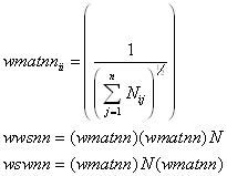
where N represents the aggregated neighbor spatial weighting matrix. As both wwsnn and wswnn have the same eigenvalues (see Ord (JASA, 1975)), using one form or another in a particular circumstance may have advantages. For example, using the symmetric form wswnn saves time in computing the log-determinants while the row-stochastic form wwsnn has some nice smoothing interpretations (the row-stochastic form constitutes a two-dimensional linear filter).
FOLS1
Syntax
[alphamax,loglik,emax,bmax,likratios,prhigher]=fols1(xsub,y)
Input Arguments
| xsub | n by p matrix where n represents the number of observations and p represents the number of non-constant independent variables |
| y | n element vector containing observations on the dependent variable |
Output Arguments
| alphamax | 0 by definition |
| loglik | (k+1) element vector of log-likelihoods. The first element is the unrestricted model log-likelihood followed by the k respective delete-1 variable subset restricted log-likelihoods |
| emax | n element vector of the errors from the OLS prediction |
| bmax | k element vector of OLS parameter estimates with the intercept as the last element |
| likratios | k element vector of twice difference between the unrestricted log-likelihood from the overall model and the k delete-1 variable subset restricted log-likelihoods. This is really the deviance (-2log(LR)). Individually these have a chi-squared distribution with 1 degree-of-freedom under the null hypothesis of no effect. |
| prhigher | k element vector of the estimated probability of obtaining a higher chi-squared test statistic under the null hypothesis of no effect. |
Description
This is a standard OLS routine with the exception of using likelihood ratio test statistics instead of t test statistics. This makes it easier to compare with the output from the various spatial routines.
FPAR1
Syntax
[alphamax,loglik,emax,bmax,likratios,prhigher]=fpar1(xsub,y,detvalz,wws)
Input Arguments
| xsub | n by p matrix where n represents the number of observations and p represents the number of non-constant independent variables |
| y | n element vector containing observations on the dependent variable |
| detvalz | iter by 2 matrix
containing the grid of values for the autoregressive parameter a
in column 1 and the associated values of |
| wws | n by n spatial weighting matrix (usually row-stochastic) |
Output Arguments
| alphamax | |
| loglik | iter by (k+1) matrix of profile likelihoods over the iter grid of values for a . The first column is the unrestricted model profile log-likelihood, followed by p respective delete-1 variable subset restricted profile log-likelihoods, and ending with the no intercept restricted profile log-likelihood |
| emax | n element vector of the errors from autoregressive model prediction |
| bmax | k element vector of model parameter estimates |
| likratios | k element vector of twice difference between the unrestricted log-likelihood from the overall model and the subset restricted log-likelihoods. For the non-constant variables the relevant restricted model corresponds to deleting a variable and its spatial lag. This is really the deviance (-2log(LR)). Hence, these have a chi-squared distribution with 1 degree-of-freedom under the null hypothesis of no effect. |
| prhigher | k element vector of the estimated probability of obtaining a higher chi-squared test statistic under the null hypothesis of no effect |
Description
This function fits the model ![]() where D represents an n
by n spatial weight matrix. The autoregressive model prediction is
where D represents an n
by n spatial weight matrix. The autoregressive model prediction is ![]() .
.
FSAR1
Syntax
[alphamax,loglik,emax,bmax,likratios,prhigher]=fsar1(xsub,y,detvalz,wws)
Input Arguments
| xsub | n by p matrix where n represents the number of observations and p represents the number of non-constant independent variables |
| y | n element vector containing observations on the dependent variable |
| detvalz | iter by 2 matrix
containing the grid of values for the autoregressive parameter a
in column 1 and the associated values of |
| wws | n by n spatial weighting matrix (usually row-stochastic) |
Output Arguments
| alphamax | |
| loglik | iter by (k+1) matrix of profile likelihoods over the iter grid of values for a . The first column is the unrestricted model profile log-likelihood followed by the respective delete-1 variable subset restricted profile log-likelihoods |
| emax | n element vector of the errors from SAR prediction |
| bmax | k element vector of SAR parameter estimates |
| likratios | k element vector of twice difference between the unrestricted log-likelihood from the overall model and the k delete-1 variable subset restricted log-likelihoods. Hence, this is really the deviance (-2log(LR)). Individually these have a chi-squared distribution with 1 degree-of-freedom under the null hypothesis of no effect. |
| prhigher | k element vector of the estimated probability of obtaining a higher chi-squared test statistic under the null hypothesis of no effect |
Description
For the simultaneous autoregression model (SAR), ![]() where D
represents a spatial weight matrix. The SAR prediction is
where D
represents a spatial weight matrix. The SAR prediction is ![]() and
hence
and
hence ![]() . The SAR prediction is not BLUP, but does have a smoothing
interpretation.
. The SAR prediction is not BLUP, but does have a smoothing
interpretation.
FSIMCAR1
Syntax
[rvcorr]= fsimcar1(wsw,rv,truerho)
Input Arguments
| truerho | scalar parameter |
| rv | n by iter matrix of independent normal random variates |
| wsw | Symmetric n by n spatial weighting matrix D |
Output Arguments
| rvcorr | n by iter matrix of CAR random variates |
Description
This generates random variates that obey the assumptions of the CAR model. The routine is more efficient (until it hits bottlenecks) with larger values of iter, which also increase memory usage. For very large n or iter, storing the Cholesky triangle and backsolving for new batches of CAR random variates would improve performance.
FSIMMIX1
Syntax
[rvcorr,invxbeta]= fsimmix1(wsw,rv,truerho,xbeta)
Input Arguments
| truerho | scalar parameter |
| rv | n by iter matrix of independent normal random variates |
| wsw | Symmetric n by n spatial weighting matrix D |
| xbeta | n element vector
containing true |
Output Arguments
| rvcorr | n by iter matrix of mixed model random variates |
| invxbeta | n element vector
containing |
Description
This generates random variates that obey the assumptions of the mixed model. The routine is more efficient (until it hits bottlenecks) with larger values of iter, which also increase memory usage. For very large n or iter, storing the Cholesky triangle and backsolving for new batches of mixed model random variates would improve performance. This routine can be used to simulate autoregressive models as well.
FSIMSAR1
Syntax
[rvcorr]= fsimsar1(wsw,rv,truerho)
Input Arguments
| truerho | scalar parameter |
| rv | n by iter matrix of independent normal random variates |
| wsw | Symmetric n by n spatial weighting matrix D |
Output Arguments
| rvcorr | n by iter matrix of SAR random variates |
Description
This generates random variates that obey the assumptions of the SAR model. The routine is more efficient (until it hits bottlenecks) with larger values of iter, which also increase memory usage. For very large n or iter, storing the Cholesky triangle and backsolving for new batches of SAR random variates would improve performance.