Spatial Statistics and Real Estate
By
R. Kelley Pace
LREC Chair of Real Estate
Department of Finance
E.J. Ourso College of Business Administration
Louisiana State University
Baton Rouge, LA 70803
(225)-388-6256
FAX: (225)-388-6366
kelley@spatial-statistics.com
kelley@pace.am
Ronald Barry
Associate Professor of Statistics
Department of Mathematical Sciences
University of Alaska
Fairbanks, Alaska 99775-6660
(907)-474-7226
FAX: (907)-474-5394
FFRPB@uaf.edu
C.F. Sirmans
Director, Center for Real Estate and Urban Economic Studies
University of Connecticut
368 Fairfield Road, U-41RE
Storrs, CT 06269-2041
(860) 486-3227
FAX: (860) 486-0349
cf@sba.uconn.edu
This manuscript appeared as,
Pace, R. Kelley, Ronald Barry, and C.F. Sirmans, "Spatial Statistics and Real Estate," Journal of Real Estate Finance and Economics, Volume 17, Number 1, 1998, p. 5-13.
(contact data has been updated since publication and a misspelling corrected)
Kluwer Academic Publishers owns the copyright to this work and has graciously granted permission to us to place this upon our website and Spatial Statistics CD-ROM.
The authors gratefully acknowledge the research support they have received from their respective institutions. We would also like to thank Jennifer Pike and Carlos Slawson.
Abstract
Real estate has historically employed statistical tools designed for independent observations while simultaneously noting the violation of these assumptions in the form of clustering of same sign residuals by neighborhood, along roads, and near facilities such as airports. Spatial statistics takes these dependencies into account to provide more realistic inference (OLS has biased standard errors), better prediction, and more efficient parameter estimation. This article provides an overview of the field and directs readers to the relevant literature and software.
Keywords: spatial statistics, CAR, SAR, kriging.
Spatial Statistics and Real Estate
Economic models in real estate often explicitly consider locational effects. Such models may differ from their spaceless counterparts. For example, the spaceless paradigm of perfect competition, as strictly interpreted, changes with the addition of transportation costs among locations.
Despite the importance of locational considerations to real estate in theory, empirical practice has employed relatively "spaceless" statistical tools, despite frequent mentions in the literature of observed violations of the assumptions underlying the optimality of such tools. For example, observing clusters of residuals of a one sign or another by neighborhood, along roads, or waterways violates the independent observation assumption underlying OLS, the most common tool in the field.
Assume the model,
![]()
\* MERGEFORMAT ()1
where Y represents the dependent variable, X represents the independent
variables, and ![]() represents the unknown, true errors. Ideally,
represents the unknown, true errors. Ideally, ![]() and thus
and thus ![]() , the
conditional mean, equals
, the
conditional mean, equals ![]() . As a sufficient
condition, if
. As a sufficient
condition, if ![]() is a normal iid random variable, X is
non-stochastic, and
is a normal iid random variable, X is
non-stochastic, and ![]() is
linear-in-the-parameters, OLS becomes normal maximum likelihood, the best linear unbiased
estimator (BLUE).
is
linear-in-the-parameters, OLS becomes normal maximum likelihood, the best linear unbiased
estimator (BLUE).
Spatial statistics has two ways to work with spatial data to make it fit the mold of
the above model. First, one can specify ![]() sufficiently well so that the residuals appear patternless over space. Second, one can
model the possible dependence of the true errors
sufficiently well so that the residuals appear patternless over space. Second, one can
model the possible dependence of the true errors![]() . We discuss both
of these routes in turn.
. We discuss both
of these routes in turn.
1. Modeling m (X)
Modelers often add regressors such as distance to various centers, indicator variables
for parts of the urban area, and so forth to help specify ![]() . Unfortunately, such models still do not usually yield patternless
residuals over space. For example, Belsley, Kuh, and Welsch (1980, p. 239) noted the
spatial clustering of residuals from the well-known hedonic pricing study of Harrison and
Rubinfeld (1978), despite the inclusion in this work of two variables measuring distances
and an indicator variable.
. Unfortunately, such models still do not usually yield patternless
residuals over space. For example, Belsley, Kuh, and Welsch (1980, p. 239) noted the
spatial clustering of residuals from the well-known hedonic pricing study of Harrison and
Rubinfeld (1978), despite the inclusion in this work of two variables measuring distances
and an indicator variable.
A moment’s reflection will show part of the problem in specifying ![]() with a few variables. As an analogy, one would
probably not attempt to cure time series problems with just a time trend term and an
indicator variable or two. In fact, the standard practice in modeling
with a few variables. As an analogy, one would
probably not attempt to cure time series problems with just a time trend term and an
indicator variable or two. In fact, the standard practice in modeling ![]() for time series requires an indicator variable
for each year. As space is two-dimensional and time is one-dimensional, if time series
analysis requires m terms, spatial data analysis would require m2
terms.
for time series requires an indicator variable
for each year. As space is two-dimensional and time is one-dimensional, if time series
analysis requires m terms, spatial data analysis would require m2
terms.
Alternatively, if one believes each neighborhood has its own effect, one would need a separate indicator variable for each neighborhood. For real estate transactions data, a typical neighborhood or subdivision might have 10-20 houses turnover in a year. This would argue for having roughly n/20 indicator variables, where n is the sample size. Hence, a data set with 10,000 observations might have 500 indicator variables. Such a large number of regressors conflicts with the natural desire for parsimonious models.
For specifying ![]() , spatial statistics has
employed several techniques. The crudest and least satisfactory technique uses a
polynomial expansion in both the east-west and north-south coordinates of each
observation’s location. This creates a two-dimensional, smooth surface. Polynomials,
while easy-to-use, suffer from several defects. First, polynomials change their global fit
based upon local errors and hence are not very robust. Hence, high degree polynomials can
"oscillate." Second, they impose more smoothness than probably desired in an
urban setting where features such as roads and natural barriers may lead to rapid changes
over space. Third, the inclusion of a large number of polynomials typically exacerbates
multicollinearity.
, spatial statistics has
employed several techniques. The crudest and least satisfactory technique uses a
polynomial expansion in both the east-west and north-south coordinates of each
observation’s location. This creates a two-dimensional, smooth surface. Polynomials,
while easy-to-use, suffer from several defects. First, polynomials change their global fit
based upon local errors and hence are not very robust. Hence, high degree polynomials can
"oscillate." Second, they impose more smoothness than probably desired in an
urban setting where features such as roads and natural barriers may lead to rapid changes
over space. Third, the inclusion of a large number of polynomials typically exacerbates
multicollinearity.
The use of splines can cure some of the problems presented by polynomials. Splines can model local behavior without changing the global fit. The user can control the amount of smoothing. In this issue, Colwell illustrates the benefits of two-dimensional splines. He presents a very intuitive, geometric development of splines and provides some natural real estate interpretations for these. His contribution illustrates the potential for more creative two-dimensional modeling of the hedonic price surface than by just using the traditional dummy and distance-based variables.
2. Modeling e
Most of the effort in spatial statistics has gone into modeling the dependence of
errors among different locations. The n by n variance-covariance matrix ![]() expresses such a dependence where
expresses such a dependence where ![]() represents
the covariance of the ith and jth errors. Ex-ante, the magnitude of
the covariance between any two errors
represents
the covariance of the ith and jth errors. Ex-ante, the magnitude of
the covariance between any two errors ![]() and
and ![]() declines as distance (under some metric) increases between location i
and location j. If the covariance depends strictly upon the distance between two
observations (relative position) and not upon their absolute position, the errors are isotropic.
Violation of this leads to anisotropy, a more difficult modeling problem. Just as
in time series, stationarity is important.
declines as distance (under some metric) increases between location i
and location j. If the covariance depends strictly upon the distance between two
observations (relative position) and not upon their absolute position, the errors are isotropic.
Violation of this leads to anisotropy, a more difficult modeling problem. Just as
in time series, stationarity is important.
As detailed below, the means of modeling the estimated variance-covariance matrix or functions of the estimated variance-covariance matrix distinguishes many of the strands of the spatial statistics literature.
Given an estimated variance-covariance matrix ![]() , one could compute
an estimated generalized least squares (EGLS) estimate.
, one could compute
an estimated generalized least squares (EGLS) estimate.
![]()
\* MERGEFORMAT ()2
The maximum likelihood estimate appears similar but introduces a log-determinant term which penalizes the use of more singular estimated variance-covariance matrices.
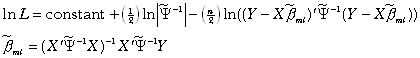
\* MERGEFORMAT ()3
If one uses a sum-of-squared error criteria alone in computing the estimates ![]() , minimization algorithms can create pathological results. To illustrate
the source of this problem, consider the effects of employing
, minimization algorithms can create pathological results. To illustrate
the source of this problem, consider the effects of employing ![]() comprised of all ones. Premultiplication of Y and X
by this matrix would result in a vector and a matrix of constants. The associated
regression would display 0 error. Naturally,
comprised of all ones. Premultiplication of Y and X
by this matrix would result in a vector and a matrix of constants. The associated
regression would display 0 error. Naturally, ![]() is singular in this case. The log-determinant term correctly penalizes such volume
reducing transformations.
is singular in this case. The log-determinant term correctly penalizes such volume
reducing transformations.
Misspecifying the variance-covariance matrix results in loss of efficiency, predictive accuracy, and biased inference. In the case of positive spatial autocorrelation, the OLS standard errors have a downward bias. Since the true information content in the dependent observations is less than in the same number of independent observations, OLS overstates the precision of its estimates.
A. Lattice Models
A set of observations located on a plane forms a lattice. Lattice models directly
approximate ![]() in the case of conditional
autoregressions or
in the case of conditional
autoregressions or ![]() in the case of
simultaneous autoregressions or models with lagged spatial dependent variables.
Frequently, (CAR) specifies
in the case of
simultaneous autoregressions or models with lagged spatial dependent variables.
Frequently, (CAR) specifies ![]() and SAR specifies
and SAR specifies ![]() , where C, D represent spatial weight matrices and
, where C, D represent spatial weight matrices and ![]() represent the relevant autoregressive parameters. Positive
represent the relevant autoregressive parameters. Positive ![]() correspond to asserting some form of direct
dependency exists between observation i and j. One can determine which
correspond to asserting some form of direct
dependency exists between observation i and j. One can determine which ![]() >0 through cardinal distance or through
ordinal distance (e.g., the four closest neighbors). Typically, C and D
have zeros on the diagonal and are non-negative matrices. In addition, C must
possess symmetry. The zeros on the diagonal means that observations are not used to
predict themselves. Hence, lattice models do not attempt to exactly interpolate (exhibit
zero error at all the sample points).
>0 through cardinal distance or through
ordinal distance (e.g., the four closest neighbors). Typically, C and D
have zeros on the diagonal and are non-negative matrices. In addition, C must
possess symmetry. The zeros on the diagonal means that observations are not used to
predict themselves. Hence, lattice models do not attempt to exactly interpolate (exhibit
zero error at all the sample points).
Often the rows of D sum to 1 (row-stochastic) which gives them a filtering
interpretation. Hence, DY would contain the average value of the neighboring Y
for each observation. For row-stochastic matrices, the log-determinants ![]() will be defined for autoregressive parameters
less than 1.
will be defined for autoregressive parameters
less than 1.
In real estate terms, the adjustment grid method represents a form of a lattice model
with ![]() and
and ![]() based upon prior information.
Pace and Gilley (forthcoming) show that SAR generalizes the usual spaceless statistical
model estimated by OLS and the grid adjustment model (c.f. Colwell, Cannaday, and
Wu (1983)). Hence, lattice models subsume the two basic paradigms of real estate empirical
work. Thus, lattice models seem naturally suited for real estate.
based upon prior information.
Pace and Gilley (forthcoming) show that SAR generalizes the usual spaceless statistical
model estimated by OLS and the grid adjustment model (c.f. Colwell, Cannaday, and
Wu (1983)). Hence, lattice models subsume the two basic paradigms of real estate empirical
work. Thus, lattice models seem naturally suited for real estate.
Interestingly, Papadakis (1937) proposed an estimator for agricultural experiment plot data extremely similar to the additive grid adjustment estimator based upon the OLS estimates of the characteristic values. Essentially, it uses information on the neighboring plots to control for microvariations in fertility just as the grid adjustment estimator uses neighboring houses to control for neighborhood variations. See Cressie (1993) or Ripley (1981) for more details on the Papadakis estimator.
Lattice models have close analogs in time series. For example, SAR models subtract the
average of the surrounding observations (scaled by the autoregressive parameter ![]() ) from each observation. This resembles the
operation in time series of subtracting from an observation the previous observation
scaled by an autoregressive constant (e.g.,
) from each observation. This resembles the
operation in time series of subtracting from an observation the previous observation
scaled by an autoregressive constant (e.g., ![]() ,
, ![]() ). As the log-determinant is equal to 0 when dealing strictly with past
data, the term does not present the same challenge for time series analysis as it does for
spatial statistics. However, spatial statistics has the advantage of having observations
in different directions near each observation while time series always deals with purely
past data. Hence, the greater symmetry and additional observations around each observation
aids spatial statistics relative to the fundamental asymmetry of time series analysis.
). As the log-determinant is equal to 0 when dealing strictly with past
data, the term does not present the same challenge for time series analysis as it does for
spatial statistics. However, spatial statistics has the advantage of having observations
in different directions near each observation while time series always deals with purely
past data. Hence, the greater symmetry and additional observations around each observation
aids spatial statistics relative to the fundamental asymmetry of time series analysis.
Real estate data sets often involve many thousands of observations. As C and D
are n by n matrices, computing the log-determinants (![]() ) would be infeasible via ordinary methods. In other work, Pace
and Barry (1997a,b) have shown how to quickly compute these log-determinants for large
data sets. For example, Pace and Barry (1997a) compute a SAR using 20,640 observations on
housing prices in California.
) would be infeasible via ordinary methods. In other work, Pace
and Barry (1997a,b) have shown how to quickly compute these log-determinants for large
data sets. For example, Pace and Barry (1997a) compute a SAR using 20,640 observations on
housing prices in California.
In this issue, Pace, Barry, Clapp, and Rodriguez use spatio-temporal lattice techniques. They condition upon previous observations which simplifies the determinant term but use averages of properties in the neighborhood which simplifies the asymmetric time series problem. Naturally, transactional price data arises over time and space and so such spatio-temporal modeling has wide application in real estate.
In addition, Prucha and Kelejian use the generalized method of moments to finesse the problems presented by the computational difficulties of the log-determinant term in estimating lattice models. GMM have seen wide application to a variety of econometric problems in recent years. Hence, the extension of GMM to spatial models opens many possibilities for jointly modeling other econometric features of the data and space.
B. Geostatistical Models
Effectively, geostatistical models directly estimate the variance-covariance matrix.
Geostatistical techniques, such as Kriging (named after Krige, a South African mining
engineer) rely upon an estimated variance-covariance matrix, ![]() ,
followed by EGLS (estimated generalized least squares), and BLUP (best linear unbiased
prediction). The simplest case assumes one can specify correctly the variance-covariance
matrix as a function of distance only (isotropy). The most typical application involves
the smooth interpolation of a surface at points other than those measured. Usually, the
method assumes errors are 0 at the measured points but modifications allow for measurement
errors at the measured points.
,
followed by EGLS (estimated generalized least squares), and BLUP (best linear unbiased
prediction). The simplest case assumes one can specify correctly the variance-covariance
matrix as a function of distance only (isotropy). The most typical application involves
the smooth interpolation of a surface at points other than those measured. Usually, the
method assumes errors are 0 at the measured points but modifications allow for measurement
errors at the measured points.
The first step in most geostatistical models is to estimate the variance-covariance matrix. While techniques exist to perform this directly, the most common technique involves the intermediate stage of computing the variogram.
The empirical variogram begins with the pair-wise squared differences among all errors (or sometimes a sample of errors for large data sets) plotted against the distance between the elements of the pair. Positively correlated errors will show small pair-wise squared differences while almost independent errors will show larger differences. For positively correlated residuals, the empirical variogram tends to start off low at small distances and rise with distance up to a point where it levels off. From the variogram one can estimate the parameters of fitted variogram functions. If the process is stationary, an equivalence exists between the fitted variogram functions and fitted covariance functions. Only a relatively small number of valid covariance functions exist which yield guaranteed positive definite estimated variance-covariance matrices (Bailey and Gatrell (1995, p. 178-181)).
Given a variogram, one can compute the kriging predictions. Note, kriging usually attempts to exactly interpolate. Hence, kriging fits perfectly (0 error) all the points in the sample. Naturally, only in rare circumstances would kriging fit perfectly the ex-sample points.
In this issue, we have two clearly written applications of geostatistical estimators to real estate. Dubin applies geostatistical techniques to real estate price data from Baltimore and in the process motivates the advantages of employing spatial statistics. As an illustration of the results, she finds kriging reduced the sum-of-squared ex-sample errors by 38% relative to OLS. Basu and Thibodeau apply geostatistical techniques to house prices in Dallas. They partition the Dallas market into eight sub-markets and apply spatial statistics to each one separately. They find spatial statistical techniques improved over OLS for six of the eight sub-markets. Interestingly, the extent of the estimated spatial error dependencies and hence the relative performance of kriging vis-ŕ-vis OLS varied substantially by submarket.
3. Spatial Statistics Software
The availability of easy-to-use spatial statistical software has been steadily increasing over the last few years. For example, SpaceStat has the most estimators, tests, and other features for lattice models. Also, S+SpatialStats, available from Mathsoft, implements lattice model estimators. Pace and Barry have a spatial statistics toolbox written in the Matlab matrix programming language which specifically attacks the computational problems associated with large data sets. See Anselin and Hudak (1992) for a review of lattice model software and implementations of lattice models in popular statistical packages.
For geostatistical estimators, the previously mentioned S+SpatialStats provides strong support. In SAS, PROC MIXED allows the specification of spatial variance-covariance matrices. In addition, many other packages such as GSLIB and GEOEAS serve this market. Pace and Barry provide Matlab programs to perform kriging for large data sets. Also for Matlab, the Mapping Toolbox contains some kriging functions and Lafleur and Gatton at University of Quebec have a kriging toolbox. In this issue, Dubin provides the code she wrote in Gauss to perform estimation.
4. Conclusion
Real estate and spatial statistics naturally complement each other. Historically, the difficulties of applying spatial statistics have limited its scope and appeal. The advances in computing, algorithms, and software have begun to make its routine application possible. The huge volume of real estate data, the large number of hypotheses of interest, and the rich heuristics accumulated by appraisers and others over the years combine to make real estate potentially one of the foremost applied areas for spatial statistics.
Employing spatial statistical estimators provides some benefits over ignoring the dependencies in the data. First, prediction can improve markedly. Using the errors on comparable properties can help hone the prediction on the subject property. Second, the estimators provide better inference as OLS yields downwardly biased standard errors in the presence of positive autocorrelation. Third, the local spatial errors (or spatially lagged variables as used with mixed regressive spatially autoregressive estimators) effectively proxy for omitted variables correlated with location. Hence, spatial statistical methods may yield different estimates for various effects than estimators which handle location in a cruder fashion.
For example, part of the difficulty of empirically studying the effects of race lies in the plethora of omitted variables present in all data. If observable variables such as race covary with difficult-to-quantify variables such as local amenities, this biases the measurement and complicates the interpretation of the regression coefficient associated with the racial variable. Similar considerations apply to studies attempting to measure the effects of pollution. In fact, Gilley and Pace (1997) found regression coefficients associated with both the racial and pollution variables fell after incorporating spatial information.
More normatively, automated appraisal, site selection, and credit scoring could benefit from the use of spatial statistical techniques. Improved methods in any of these areas could provide substantial benefits to innovative firms.
Fortunately, real estate has already begun to take advantage of spatial statistics. In addition to the previously discussed papers, Goetzmann and Spiegel (1997) as well as Can and Megbolugbe (1997) employed spatial statistical methods in their empirical work in a recent issue of this journal. Also, Gelfand, Ghosh, Knight, and Sirmans (forthcoming) have applied the Gibbs sampler to compute Bayesian estimates for a lattice model. These represent only the beginning of a series of new papers which will truly integrate real estate spatial considerations and empirical work.
Finally, as encouragement to our readers to become involved in these developments, in Table 1 we list a number of good spatial statistics reference sources, seminal articles, and introductory texts.
Table 1 — Some Spatial Statistics Selections |
|
| Anselin (1988) | This provides the most detailed exposition of simultaneously specified lattice models from a geographic and econometrics perspective. |
| Anselin and Hudak (1992) | Good description of the basic estimation problem. This appears in a special issue containing a number of interesting articles. |
| Bailey and Gatrell (1995) | This is the easiest, albeit limited, introduction to the various spatial statistical methods. As a bonus, the text comes with DOS software for estimating some of the models. |
| Colwell, Cannaday, and Wu (1983) | The first paper to formalize real estate’s homegrown spatial statistical estimator, the grid adjustment method. |
| Cressie (1993) | This voluminous text treats both lattice and geostatistical models and serves as a standard reference for the field. |
| Dubin (1988) | This provides one of the clearest expositions of spatial statistical estimation. |
| Goldberger (1962) | The easiest-to-read derivation of best linear unbiased prediction (BLUP) from an econometric perspective and notation. |
| Griffith (1992) | An interesting, non-technical discussion of the various causes and implications of spatial autocorrelated data. |
| Haining (1990) | A well-written, comprehensive survey of the field. Inexpensive. |
| Ord (1975) | The starting point for most geographical lattice modeling. |
| Papadakis (1937) | A parallel development to the grid estimator used in the analysis of agricultural field experiments. |
| Ripley (1981) | This develops SAR and CAR lattice models as well as geostatistical ones. A standard reference in the field. |
Bibliography
Anselin, Luc, Spatial Econometrics: Methods and Models, Dordrecht: Kluwer Academic Publishers, 1988.
Anselin, Luc, and S. Hudak, "Spatial Econometrics in Practice: A Review of Software Options," Journal of Regional Science and Urban Economics, 22 (1992), 509-536.
Bailey T., and A. Gatrell, Interactive Spatial Data Analysis, Harlow: Longman, 1995.
Barry, Ronald, and R. Kelley Pace, "Kriging with Large Data Sets Using Sparse Matrix Techniques," Communications in Statistics: Computation and Simulation, Volume 26, Number 2, 1997, p. 619-629.
Belsley, David, Edwin Kuh, and Roy Welsch, Regression Diagnostics, New York: Wiley, 1980.
Can, Ayse, and Isaac Megbolugbe, "Spatial Dependence and House Price Index Construction," Journal of Real Estate Finance and Economics, 14, (1997), p. 203-222.
Colwell, Peter F, Roger E. Cannaday, and Chunchi Wu. "The Analytical Foundations of Adjustment Grid Methods." Journal of the American Real Estate and Urban Economics Association 11 (1983), 11-29.
Cressie, Noel A.C., Statistics for Spatial Data, Revised ed. New York: John Wiley, 1993.
Dubin, Robin A. "Estimation of Regression Coefficients in the Presence of Spatially Autocorrelated Error Terms." Review of Economics and Statistics, 70 (1988), 466-474.
Gelfand, Alan E., Sujit K. Ghosh, John R. Knight and C.F. Sirmans. "Spatio-Temporal Modeling of Residential Sales Data." Journal of Business and Economic Statistics (forthcoming).
Goetzmann, William and Matthew Spiegel, "A Spatial Model of Housing Returns and Neighborhood Substitutability," Journal of Real Estate Finance and Economics, 14, (1997), p. 203-222.
Goldberger, Arthur, "Best Linear Unbiased Prediction in the Generalized Linear Regression Model," Journal of the American Statistical Association, (1962).
Griffith, Daniel A., "What is Spatial Autocorrelation?," L’Espace Géographique, Volume 3, 1992, p. 265-280.
Haining, Robert, Spatial Data Analysis in the Social and Environmental Sciences, Cambridge, 1990.
Harrison, D. and D. L. Rubinfeld, "Hedonic Prices and the Demand for Clean Air," Journal of Environmental Economics and Management, 5, (1978), p. 81-102.
Ord, J.K., "Estimation Methods for Models of Spatial Interaction," Journal of the American Statistical Association, 70 (1975), p. 120-126.
Pace, R. Kelley, and Ronald Barry, "Quick Computation of Regressions with a Spatially Autoregressive Dependent Variable," Geographical Analysis, Volume 29, Number 3, July 1997, p. 232-247.
Pace, R. Kelley, and O.W. Gilley, "Using the Spatial Configuration of the Data to Improve Estimation," Journal of the Real Estate Finance and Economics, Volume 14, Number 3, 1997, p. 333-340.
Pace, R. Kelley, and O.W. Gilley, "Optimally Combining OLS and the Grid Estimator," Real Estate Economics, forthcoming
Pace, R. Kelley, and Ronald Barry, "Sparse Spatial Autoregressions," Statistics and Probability Letters, Volume 33, Number 3, May 5 1997, p. 291-297.
Papadakis, J. S., "Méthode Statistique pour des Expériences sur Champ," Bull. Inst. Amel. Plantes a Solonique, 23, 1937.
Ripley, Brian D. Spatial Statistics. New York: John Wiley, 1981.